The basics of radial velocities¶

We can almost completely characterize the orbits of massive bodies around a star using a set of five orbital parameters for each body. Different parametrization schemes use a different set of five parameters, depending on what kind of optimization is needed, but for this tutorial we will use the one from Murray & Correia (2010):

\(K\): radial velocity semi-amplitude
\(T\): orbital period
\(e\): eccentricity of the orbit
\(\omega\): argument of periapse
\(t_0\): time of periapse passage

These parameters exist for each body orbiting a star.

In this notebook, we will play around with the package radial to simulate radial velocity curves for a star orbited by bodies with different orbital parameters.

from radial import body
import astropy.units as u
import numpy as np
import matplotlib.pyplot as plt

Let’s start with a very familiar object: the Sun.

Note: if you are too lazy to convert units like me, I recommend using the astropy.units module.

sun = body.MainStar(mass=1 * u.solMass, name='Sun')

Now let’s setup a couple of companions for the Sun. How about Earth and Jupiter?

Thei radial velocity semi-amplitude is not easily accessible from online databases, but we can compute them using the following equation:

\[K = \frac{m \sin{I}}{m + M} \frac{2\pi}{T} \frac{\ a}{\sqrt{1-e^2}} \mathrm{,}\]

where \(m\) is the companion mass, \(M\) is the mass of the main star, \(I\) is the inclination angle between the reference plane and the axis of the orbit (let’s consider \(I = \pi / 2\) in this example) and \(a\) is the semi-major axis of the orbit. All these parameters are easily accessible to us.

def compute_k(mass, period, semia, ecc, i=np.pi * u.rad):
    return mass / (mass + 1 * u.solMass) * 2 * np.pi / period * semia / (1 - ecc ** 2) ** 0.5

# Computing K for the Earth
mass_e = 1 * u.earthMass
semia_e = 1.00000011 * u.AU
period_e = 1 * u.yr
ecc_e = 0.01671022
k_e = compute_k(mass_e, period_e, semia_e, ecc_e)

# Computing K for Jupiter
mass_j = 1 * u.jupiterMass
semia_j = 5.2026 * u.AU
period_j = 11.8618 * u.yr
ecc_j = 0.048498
k_j = compute_k(mass_j, period_j, semia_j, ecc_j)

# Setting up the companions
earth = body.Companion(main_star=sun,
                         k = k_e,
                         period_orb=period_e,
                         t_0=2457758.01181 * u.d,    # Time of periastron passage, Julian Date
                         omega=114.207 * u.deg,      # Argument of periapsis/perihelion
                         ecc=ecc_e)

jupiter = body.Companion(main_star=sun,
                           k=k_j,
                           period_orb=period_j,
                           t_0=2455636.95833 * u.d,
                           omega=273.867 * u.deg,
                           ecc=ecc_j)

The next step is to setup the Solar System with the Sun and its planetary companions. We need to state what is the time window that we want to simulate in Julian Dates.

time = np.linspace(2453375, 2457758, 1000) * u.d    # ~12 years

# The Solar System
sys = body.System(main_star=sun,
                    companion=[earth, jupiter],
                    time=time)

Now to compute the radial velocities of the Sun due to Earth and Jupiter:

sys.compute_rv()

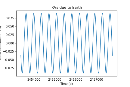
With the radial velocities finally computed, it’s time to plot them. Let’s take a look at the RVs caused by the Earth on the Sun:

sys.plot_rv(0, 'RVs due to Earth')
plt.show()

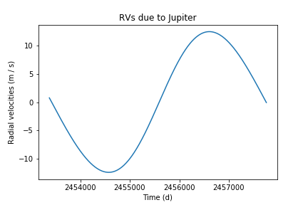
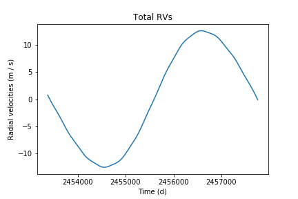
And the total RVs (including Jupiter) are shown below:

sys.plot_rv(1, 'RVs due to Jupiter')
sys.plot_rv(plot_title='Total RVs')
plt.show()